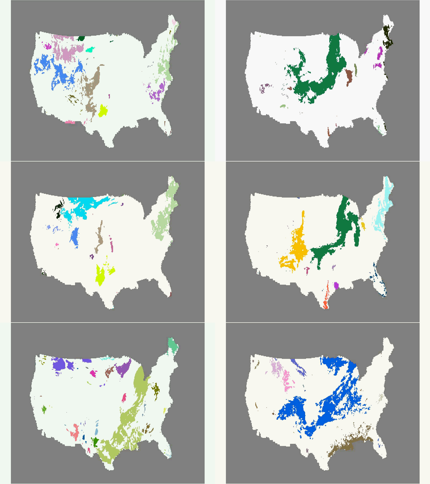
AICCA: AI-Driven Cloud Classification Atlas

Project Summary:

Clouds represent the single largest uncertainty in projections of future climate change. Their multi-scale nature means that even state-of-the-art numerical climate simulations cannot reliably project how their distribution, frequency, and properties will alter under high-CO2 conditions. Observational data may therefore be key to understanding cloud behavior, but the information contained in decades and petabytes of multispectral cloud imagery from satellite instruments has received only limited use. Recent advances in artificial intelligence (AI) now allow tapping this underutilized resource to improve understanding of cloud dynamics and feedbacks. A core requirement for analysis of cloud images is dimension reduction: dividing a complex high-resolution spatial field into a more limited set of categories. Most attempts at automated cloud classification to date have involved supervised learning of a limited number of human-defined cloud categories, but spatial patterns of cloud textures vary widely, and our goal is to produce novel classifications that provide new insight.

Clouds project therefore proposes, Rotation-Invariant Cloud Clustering (RICC), instead to leverage modern unsupervised deep learning methods to identify robust and meaningful clusters of cloud patterns, and to apply the resulting clustering method to 22 years of data from the Moderate Resolution Imaging Spectroradiometer (MODIS) instruments on NASA’s Aqua and Terra satellites. The resulting AI-driven dataset of cloud classifications, AICCA: AI-driven Cloud Classification Atlas, will deliver in a compact form (10s of GB of class labels, with high spatial and temporal resolution) information currently accessible only as 100s of TB of multi-spectral images.

AICCA will enable the data-driven diagnosis of patterns of cloud organization, provide insight into their evolution on timescales of hours to decades, and contribute to a democratization of climate research by facilitating access to core data.

For more information on the project:

https://takglobus.github.io/AICCA-explorer/

https://github.com/RDCEP/clouds

Paper Link: https://www.mdpi.com/2072-4292/14/22/5690

Paper Summary:

Clouds play an important role in the Earth’s energy budget and their behavior is one of the largest uncertainties in future climate projections. Satellite observations should help in understanding cloud responses, but decades and petabytes of multispectral cloud imagery have to date received only limited use. This study describes a new analysis approach that reduces the dimensionality of satellite cloud observations by grouping them via a novel automated, unsupervised cloud classification technique based on a convolutional autoencoder, an artificial intelligence (AI) method good at identifying patterns in spatial data.

Our technique combines a rotation-invariant autoencoder and hierarchical agglomerative clustering to generate cloud clusters that capture meaningful distinctions among cloud textures, using only raw multispectral imagery as input. Cloud classes are therefore defined based on spectral properties and spatial textures without reliance on location, time/season, derived physical properties, or pre-designated class definitions. We use this approach to generate a unique new cloud dataset, the AI-driven cloud classification atlas (AICCA), which clusters 22 years of ocean images from the Moderate Resolution Imaging Spectroradiometer (MODIS) on NASA’s Aqua and Terra instruments---198 million patches, each roughly 100 km x 100 km (128 x 128 pixels)---into 42 AI-generated cloud classes, a number determined via a newly-developed stability protocol that we use to maximize richness of information while ensuring stable groupings of patches. AICCA thereby translates 801 TB of satellite images into  54.2 GB of class labels and cloud top and optical properties, a reduction by a factor of 15000. The 42 AICCA classes produce meaningful spatio-temporal and physical distinctions and capture a greater variety of cloud types than do the 9 International Satellite Cloud Climatology Project (ISCCP) categories: for example, multiple textures in the stratocumulus decks along the West coasts of North and South America. We conclude that our methodology has explanatory power, capturing % in that it captures regionally unique cloud classes and providing rich but tractable information for global analysis. AICCA delivers the information from multi-spectral images in a compact form, enables data-driven diagnosis of patterns of cloud organization, provides insight into cloud evolution on timescales of hours to decades, and helps democratize climate research by facilitating access to core data.

People

Takuya Kurihana

Climate variability: statistics and observation based simulations

Characterizing potential future changes in temperature variability across frequencies: 

The impacts of climate change on human societies may arise not just from changes in climate means but from changes in climate variability. Many agricultural crops, for example, are highly sensitive to even brief periods of stress temperatures, particularly at certain times of the growing cycle. Crop yields can be strongly affected by changes in temperature variability even in the absence of a change in mean. Understanding potential changes in temperature variability has therefore been a research priority in climate science.

Impacts of climate variability depend on not only the magnitude but also the frequency of variations: day-to-day temperature fluctuations have different consequences than year-by-year differences. We therefore study variability using spectral methods that allow distinguishing timescales of fluctuations. Current projects address climate variability in a number of ways

• comparing variability changes in present-day or preindustrial and and future equilibrated climates
• developing methodologies to characterize variability changes in transient climates
• evaluating the effect of model spatial resolution on temperature variability

In our study of equilibrated climates, we compare pre-industrial and future climate scenarios in two different climate models, CCSM3 and GISS-E2-R, with millennial runs so that each climate state is stationary. Following techniques developed in Leeds et al (2015),  we compute integrated variability in distinct frequency bands and show changes over time as the future/present ratio. spectral ratios to explore the temperature variability changes in increased radiative forcing based on climate models. Within CCSM3, we also compare variability changes when warming is driven by two different forcing agents (CO2 and solar radiation).

Figure 1: Changes in summertime (JJA) temperature variability in three frequency bands from pre-industrial to future climates states, for Two models: (LEft) CCSM3 (289 ppm → 1400 ppm); (Right) GISS-E2-R (285 ppm → 1140 ppm). Variability changes are shown as ratios of the standard deviation, Values below 1 mean temperature variability decreases. GISS-E2-R model outputs are regrided to T31 resolution as CCSM3 using area-conserving remapping. Patterns In both models are similar: variability tends to increase slightly over land and decrease over the ocean. (In wintertime, variability tends to decrease everywhere other than tropical land.)

Characterizing and emulating variability in a transient climate:

Characterizing climate variability is easier in stationary conditions, but the Earth for the foreseeable future will be in a changing or "transient" state, in which temperatures are evolving in response to changed CO2 concentrations. Most archived climate model output also simulates transient states. We therefore seek to statistically describe how variability changes in a transient climate. This statistical exploration also serves our overall research goal is also to use model information to produce "data-driven simulations" for use in impacts assessments.  GCM output should not be used directly in impacts assessments, because GCMs do not fully reproduce present-day temperature distributions. Instead we develop methods of generating simulations of future temperatures that combine observational records with GCM projections of changes in variability (covariances). (See Figure 2 for cartoon, also description of emulation research.) 

Figure 2: Cartoon illustration comparing strategies for simulating temperatures that combine information from a model and the observational record. Columns compare simple bias correction (left), the Delta method (center), and our proposed method (right). Top row, the model predicts changes in mean temperature but no changes in variability; in this case, our proposed method is equivalent to the Delta method. Bottom row, the model predicts changes in both mean and covariance. Simple bias correction does not retain the higher order properties of the observations, whereas the Delta method does not account for model changes in covariance; our proposed method does both. FROM POPPICK ET AL, 2015.

Again using the CCSM3 model, but now an ensemble of transient simulations rather than a single stationary run, we describe a statistical model for the evolution of temporal covariances in a GCM in response to altered CO2 levels. We find that, at least in CCSM3, changes in the local covariance structure can be explained largely as a function of the regional mean change in temperature, with a small term related to the rate of change of warming. (A warming climate will have slightly greater variability than an equilibrium climate at the same temperature.)

The statistical model can then be used to emulate the evolving covariance structure of temperatures, and therefore used to create in data-driven simulations that account for the projections of changes while still retaining fidelity with the observational record. We demonstrate the emulation of variability changes below, training the statistical model on model runs of several CO2 scenarios and using it to emulate changes under another scenario. Variability changes can indeed be described and emulated with a simple statistical model.

Figure 3: (Left): ESTIMATES OF CHANGES IN VARIABILITY IN Future (year 2100) RELATIVE TO PREINDUSTRIAL CLIMATEs, UNDER A MONOTONICALLY INCREASING CO2 CONCENTRATION SCENARIO IN CCSM3. RED INDICATES AN INCREASE IN VARIABILITY AND BLUE A DECREASE IN VARIABILITY. THE ASSOCIATED TIMESCALE OF VARIATION FOR WHICH THE CHANGES IN VARIABILITY ARE DISPLAYED IS GIVEN ABOVE ON THE Y-AXIS OF THE  MAP.  (RighT):, emulation of The Estimates on the LEFT. Locations are marked with “.” (or “x”) when the difference between the emulator and the fitted model is more than two (or three) standard errors away from zero. The patterns are similar under both schemes, with most of the differences at locations where our model would not be expected to be a good description of changes in variability (e.g., at ice margins). From Poppick et al, 2015.

People: Jeremy Klavans | Liz Moyer | Andy Poppick | Michael Stein | Shanshan Sun

Alumni: William Leeds | David McInerney

Partners: Larissa Nazarenko | Gavin Schmidt

Recent Publications:

A. Poppick, D. J. McInerney, E. J. Moyer, and M. L. Stein. Temperatures in transient climates: improved methods for simulations with evolving temporal covariances. arXiv preprint arXiv:1507.00683 (2015).

W. B. Leeds, E. J. Moyer, and M. L. Stein. Simulation of future climate under changing temporal covariance structures. Advances in Statistical Climatology Meteorology and Oceanography, 1(1):1–14, 2015

Climate model emulation

The study of future climate change necessarily involves numerical simulations. However, the state-of-the-art general circulation models (GCMs) used to producing climate projections are highly computationally demanding, so that century-long model runs may take months of calendar time to complete. GCMs are therefore too unwieldy for use in many contexts, especially in policy analysis. Analyses that involve optimal policy determination or uncertainty quantification require repeated iterations of climate projections for different CO2 trajectories, something that is computationally prohibitive with GCMs. We therefore seek techniques that capture (emulate) the behavior of GCMs but in computationally leaner tools that are useful in climate impacts assessments and other policy analyses requiring rapid climate projections. 

We have developed a new approach for emulating the output of a GCM under arbitrary forcing scenarios using only a small set of precomputed runs from the model. We express temperature and precipitation are expressed as simple functions of the past trajectory of atmospheric CO2 concentrations, and fit the statistical model using a "training set" of model output (Castruccio et al, 2014). The approach captures the nonlinear evolution of climate anomalies shown in coupled climate models,  and, once the statistical model is fit, produces emulated climate output effectively instantaneously. In our 2014 paper, we demonstrated emulation of temperature and precipitation over sub-continental regions. In current work, we have extended emulation to individual model grid cells, by incorporating information about spatial correlations (Figure 1 below).

Figure 1: Improving emulation by incorporating spatial information. Figure shows model output from CCSM3 (grey, mean of five realizations) and emulations with various models (colored) for scenarios with an abrupt drop (Left) and jump (Right) in CO2 concentration.  Top And bottom rows show two different example grid cells  (A and B are in North America, C and D in central africa).  The spatio-temporal statistical model Is shown in red. the spatio-temporal emulator adequately captures temperature trends At pixel level even when CO2 IS CHANGING RAPIDLY.

 

Multi-model emulation:

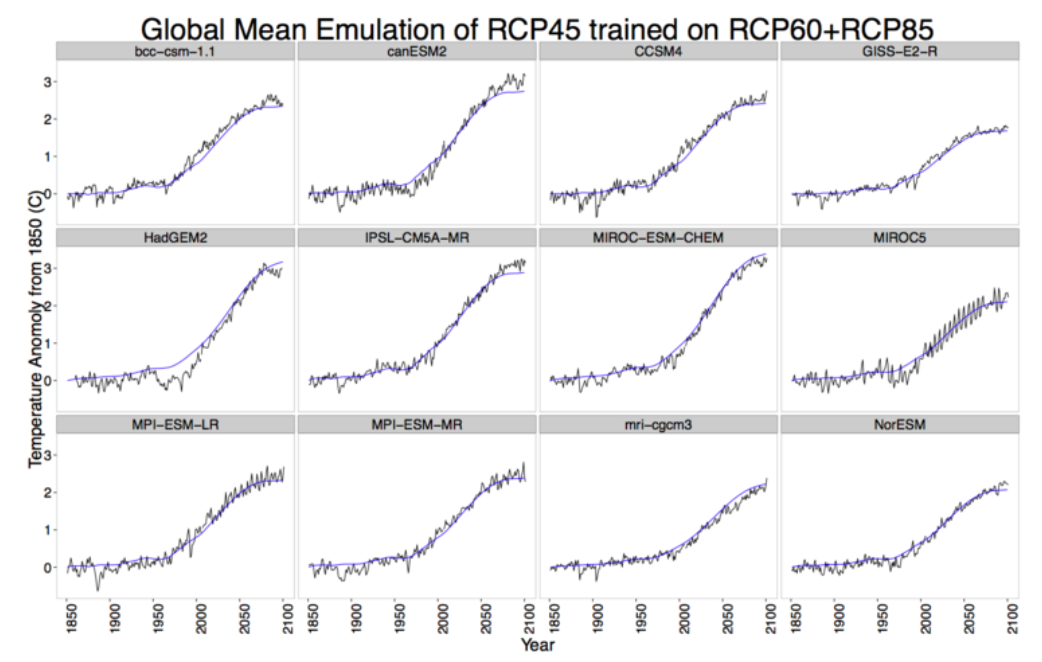
In the work described above, we demonstrate emulation on a single climate model, CCSM3, with a custom-designed training set. In current work, we are extending the technique to emulate all major state-of-the-art GCMs, using only publicly available archived model output in the CMIP5 archive.  We have tested 22 individual CMIP5 models to date; in all the simple emulation approach captures regional temperature evolution well.

Figure 2: Emulation of global mean temperature evolution FOR TWELVE GCMS under the IPCC RCP4.5 scenario of future CO2. each Model is emulated separately., with the emulator trained on model temperature output generated with the RCP60 and RCP85 CO2 scenarios. Emulation (blue) adequately captures actual GCM output (black).

Our work in multi-model emulation also includes evaluation of how small training sets can be (in terms of multiple scenarios or realizations) to maintain adequate emulation, and physical interpretation of the fitted emulation parameters for each model. These fitted parameters offer a metric with interpretable physical significance that allows us to characterize and classify climate models.

People: 

Elisabeth Moyer | Aidan Sadowski | Michael Stein | Shanshan Sun | Andrew Poppick | Jingyu Bao

Alumni:

 Feifei Liu Crouch |  William Leeds | David McInerney

Recent Publications:

Stefano Castruccio et al. "Statistical Emulation of Climate Model Projections Based on Precomputed GCM Runs*." Journal of Climate 27, no. 5 (2014): 1829-1844.

Precipitation in future climates: rainstorms

This project is aimed at characterizing changes in future precipitation suggested by climate models, and using that information along with observations to produce data-driven simulations that can be used to evaluate impacts (e.g. changes in floods, water supply, and agricultural yields).

Climate models robustly predict a rise that global rainfall will rise under warmer climate conditions, and that rain events become more intense (because a warmer atmosphere holds more water vapor). The combination also requires some third adjustment: because the projected increase in rainstorm intensity (about 6% per degree C of warming) is greater than the projected total rise in precipitation (about 3%/degree), some other aspect of precipitation in the climate models must change to compensate. Either storms are initiated less frequently, or rain events are shorter in duration, or rainstorms are smaller in extent, or some combination of these effects. To date no study has determined how exactly precipitation characteristics change, in part because of the statistical challenge of representing precipitation, a complex, non-Gaussian process with strong spatiotemporal correlations. 

We have developed a new approach to characterizing changes in precipitation in future climates that moves away from considering time series at individual locations, and instead uses image-processing algorithms to identifying individual rainstorm events and capture the evolution of storms in space-time space. The effort does require a very large volume of data: observations and model output at very high spatial resolution on time steps of a few hours or less. In this study, we use dynamically downscaled climate model output (CESM downscaled with WRF)  at 12 km, 3 hourly resolution. We compare model output to real-world precipitation estimated from weather radar: the NCEP Stage IV data product at 4 km, 1 hourly resolution.

 FIGURE 1: EXAMPLE OF RAINSTORM OBJECTS CONSTRUCTED BY OUR RAINSTORM IDENTIFICATION AND TRACKING ALGORITHM, FROM MODEL OUTPUT IN (LEFT) SUMMER AND (RIGHT) WINTER.  COLORS REPRESENT DIFFERENT IDENTIFIED RAINSTORM OBJECTS. MOVEMENT OF SAME-COLORED REGIONS SHOW EVOLUTION OF INDIVIDUAL RAINSTORMS OVER TIME. IN SUMMER, CONVECTIVE STORMS INITIATE OVER MUCH OF THE U.S., ESPECIALLY IN THE WEST. RAINFALL IN WINTER OCCURS PRIMARILY IN LARGE-SCALE STORMS.

In the model output studied, we find that storms do indeed become more intense in future climate conditions but that their initiation, duration, and trajectories are nearly unchanged. The compensating adjustment is that storms simply become smaller in spatial extent.

The goal of this work is not only improving scientific understanding but developing statistical methods for generating future precipitation scenarios that combine information from both observational data and climate model runs. That is, simulations should capture the changes shown in models but preserve the statistical characteristics of real-world rainfall.  Altering the spatial extent of rain events in data is non-trivial. Figure 2 below shows the application of a transformation algorithm applied to Stage IV radar data. In general, we hope this work will enable new ways of thinking about precipitation events in both meteorology and climatology. 

Figure 2: Example OF precipitation patterns in observations (left) and after transforming the rainstorm size and intensity (RIGHT). Red crosses represent the intensity-weighted center of individual rainstorms. To simulate the rainstorm size changes suggested by our regional climate model runs, we shrink Or enlarge each rainstorm by reducing or increasing the distance to this center from individual rainstorm pixels. After resizing, we transform the rainfall intensity time series at each location to reflect the intensity distribution changes suggested by our model runs.

People

Won Chang | V. Rao Kotamarthi | Elisabeth Moyer | Michael Stein | Jiali Wang

Recent Presentations:

• Won Chang. A conditional simulation approach to future precipitation scenario generation. Poster presented at: Data Assimilation Workshop, STATMOS Summer School. May 2015.

• Won Chang. A conditional simulation approach to future precipitation scenario generation. Poster presented at: STATMOS Annual Meeting. University of Chicago, Chicago, IL. September 2014. 

Climate extremes

Changes in U.S. temperature extremes under increased CO2 in millennial-scale climate simulations 

Changes in extreme weather may produce some of the largest societal impacts from anthropogenic climate change. (At present, weather damages are dominated by rare events that happen only every several decades or more.) However, predicting future changes in those rare events is not possible using only the short observational record.  Insight on changes in extremes must come from climate models, where we can generate long simulations.

In this project, we use millennial runs from the Community Climate System Model version 3 (CCSM3) in equilibrated pre-industrial and future (700 and 1400 ppm CO2) conditions to examine both how extremes change and how well these changes can be estimated as a function of run length.

Figure 1: Illustration of how changes in extreme TEMPERAtures can differ from changes in OVERALl temperature distributions. Model output FrOM 1000-year RUNS OF CCSM3 with CO2 at pre-industrial (PI) and 2.5 x PI (700 ppm) levels, from a mid-latitudes location (in Idaho).

(a, bottom): daily temperatures in Winter (DJF), with PI in blue and future in  RED. (B, TOP). annual cold extremes (Annual Winter TMIN), on same temperature scale. Note that Winter extreme cold TEmperatures WARM MORE strongly than The mean temperature shift. (From Huang et al, 2015)

Extreme value theory provides a means of estimating the far tails of distributions. We estimate changes to distributions of future temperature extremes by fitting annual maximum and minimum temperatures to generalized extreme value (GEV) distributions.  

Using 1000-year preindustrial and future timeseries of temperatures in the contiguous United States, we show that changes in extremes are different in summer and winter. In winter, cold extremes generally warm much more than the mean shift in wintertime temperatures (Figure 1), while in summer, warm extremes generally warm only as much as the shift in means. 

The changes in winter extremes involve more than a simple shift in magnitudes. The scale and shape of their distributions also change. This effect is best demonstrated by plotting the "return level" of extreme events, i.e. the magnitude of an extreme that recurs on a specified timescale. Figure 2 below shows changes in the 2-year to 100-year return levels for wintertime cold extremes. Over ocean regions (red lines at lower left are the Pacific off California; those on right are the Gulf of Mexico and the Atlantic), changes are relatively flat across time, suggesting a simple shift in the distribution of extremes. Over land regions, however, changes show complex behavior. In the inland Southwest U.S.,  changes in the 100-year "extreme extremes" are larger than changes in the 2-year "moderate extremes". Further north, this pattern is reversed.

FIGURE 2: ESTIMATED CHANGES IN RETURN LEVELS OF WINTER TMIN  EXTREMES IN 700 PPM CO2 VS. PRE-INDUSTRIAL MODEL RUNS FOR THE NORTH AMERICAN REGION ( 6 X 16 GRID CELLS). EACH OF THE 16 PANELS REPRESENTS A LONGITUDE; IN EACH PANEL, THE 6 LATITUDES ARE DENOTED BY COLOR. THE X AXIS OF EACH PANEL IS THE RETURN PERIOD AND Y AXIS THE CHANGE IN  RETURN LEVEL.THICK DASHED LINES SHOW ESTIMATED RETURN LEVEL CHANGES; THE ENVELOPES SHOW ASSOCIATED UNCERTAINTIES (ESTIMATED FROM BLOCK BOOTSTRAPPED SAMPLES WITH RESAMPLED YEARS).  FOR EACH GRID CELL, THE CORRESPONDING MEAN TEMPERATURE CHANGE IS MARKED WITH A SYMBOL (CROSSES FOR LAND AND BOXES FOR OCEAN LOCATIONS). (FROM HUANG ET AL., 2015.)

The 1000-year runs used here allow us to accurately determine changes in even 100-year extremes, but in practice, most modeling studies must rely on shorter runs. GEV modeling should allow estimation of infrequent events using relatively short time series, but it is important to understand its limitations for climate data. We therefore repeat the estimation of selected return levels (20-, 50-, and 100-year extremes) using segment of the timeseries of varying length. The resulting estimates can become very poor when the timeseries is of comparable length or shorter than the return period of interest: that is, a 100-year model run cannot be used to reliably estimate changes in 100-year extremes. These results suggest caution when attempting to use short observational records or model runs to infer changes in extreme events. 

People:

Whitney Huang | Elisabeth Moyer | Michael Stein | Shanshan Sun | David McInerney | Hao Zhang

Soil Moisture

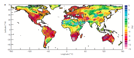
Although many impacts of climate change remain uncertain, climate models robustly project that land surfaces become drier in warmer climate conditions. General circulation models (GCMs) almost universally show reduced soil moisture over much of the globe, even in locations where average rainfall increases (Figure 1). This change is a significant societal concern both because of potential effects on food production and because drier soils feed back on local weather conditions, exacerbating heat waves. (In wetter conditions, evaporative cooling buffers extreme temperatures.) These adverse consequences make understanding the surface-atmosphere interactions that control soil moisture a research priority.

Figure 1: PROJECTED CHANGES IN SOIL MOISTURE IN THE TOP 10 CM LAYER, FROM 1980-1999 TO 2080-2099 UNDER A MODERATE EMISSIONS SCENARIO: MULTIMODEL MEAN % ChANGE FROM 11 CMIP5 MODELS. MOST LAND AREAS BECOME DRIER. From (DAI et al., 2013).

While the model projections of drying are plausible, the model representation of soil moisture dynamics have not been fully validated. Soil moisture observations are sparse and controversial, and there is as yet no consensus on whether the historical record suggests that droughts are increasing. The RDCEP soil moisture project is using a unique observational resource to characterize soil dynamics and test the representation of soil moisture in models. We make use of the Department of Energy’s Atmospheric Radiation Measurement Climate Research Facility at the Southern Great Plains site in Kansas and Oklahoma (ARM-SGP), where soil moisture, moisture fluxes, and meteorological variables have been measured at hourly intervals over more than a decade, as a test-bed for characterizing statistical relationships between soil moisture and moisture fluxes and local forcing variables (e.g. temperature, precipitation, wind speed, and relative humidity). We then compare to output from the soil moisture model (CLM) used in the Community Earth System Model, one of the most widely-used climate models, to understand how well models capture the physics controlling soil moisture.

People: 

Scott Collis |  Elisabeth Moyer | Michael Stein | Shanshan Sun 

Support: 

This project is supported in part by a University of Chicago - Argonne National Laboratory Strategic Collaboration Initiative seed grant.

Recent Presentations:

• Shanshan Sun. Statistical exploration of processes controlling soil moisture in present and future climates. Poster presented at: ARM/ASR Joint User Facility/PI Meeting, Tyson’s Corner, VA. March 16-19, 2015. 

Climate Emulator

To characterize climate change impacts in long range simulations using economic and Integrated Assessment (IA) models, we are also developing statistical emulators (i.e. response functions) that map from inputs (e.g. irrigation and fertilizer application) and atmospheric conditions (e.g. atmospheric CO2 and regional temperature and precipitation measures) to agricultural productivity measures at a variety of scales. We are developing a number of aggregation and scaling methodologies to translate high-resolution gridded products to decision-relevant environmental and political scales (e.g. county, watershed, or national boundaries). These methodologies must be versatile enough to map vulnerability, impact, and adaptation (VIA) measures to arbitrary spatial scales, while consistently tracking ensemble uncertainty information throughout.

The emulation tool provides statistical representations of the behaviors of a number of general circulation models (GCMs) from different research groups. The emulator is designed to mimic how the larger models would have responded, and can provide projections of regional temperatures for any user-chosen scenario of future CO2 concentrations.

The emulator is ‘trained’ on publicly-available model simulations of scenarios specified for the IPCC 5th Assessment Report. Users can explore emulated model responses to three IPCC scenarios (RCPs 2.6, 4.5, and 8.5) and one scenario of continuous exponential growth in CO2. Users can also upload their own CO2 scenarios.

Projecting temperature change

Comparing regions

SCREENSHOTS OF THE CLIMATE EMULATOR TOOL

---

Statistical Emulation

Statistical emulation of climate model output involves using a ‘training set’ of simulations for each model to fit the parameters of a simple statistical model that describes the climate response to changing CO2 concentrations. In the tool here, each region is fit separately.

Radiative forcing associated with the different RCP scenarios. RCP 8.5 represents 'business-as-usual'. Click here for further description

The training set used is archived GCM simulations made as part of the Coupled Model Intercomparison Project 5 (CMIP5), and archived at the Earth Systems Grid database (available from various sites, including here or here). The simulations use CO2 scenarios developed for the Intergovernmental Panel on Climate Change 5th Assessment Report. These ‘Representative Concentration Pathways’, or RCPs, describe the CO2 concentrations associated with various potential emissions scenarios (see graphic on the left). Where available, we use RCP 4.5, RCP 6.0, and RCP 8.5 as the training set. For some models that did not archive all scenarios, we use only RCP 4.5 and RCP 8.5.

The statistical model used for emulation is described in detail in Castruccio et al 2013

---

People: Alison Brizius | Nathan Matteson | Elisabeth Moyer | Aidan Sadowski | Michael Stein 

Alumni: Stefano Castruccio | Bill Leeds | John Moosemiller | Grant Wilder

Related Publications:

Stefano Castruccio et al. "Statistical Emulation of Climate Model Projections Based on Precomputed GCM Runs*." Journal of Climate 27, no. 5 (2014): 1829-1844.